Tests of Second-order Stationarity
This section assume that the trend and seasonality has been modeled and removed from your time series and you wish to test whether it is second-order stationary. Here, by TEST we mean a statistically rigorous hypothesis test. We will examine two tests here based on methods described in Priestley and Subba Rao (1969) and Nason (2013). The reason for focussing on these tests is that there are freely available implementations in the freeware programming language R. However, it is important to note that there are several other possible tests that could be used and some of them are listed in Nason (2013).
The Priestley-Subba Rao (PSR) Test
Description. The PSR test centres around the time-varying Fourier spectrum ft(w) where t is time and w is frequency. For a stationary time series the time-varying spectrum is, not surprisingly, a constant function of time. The PSR test investigates how "non-constant" ft(w) is a function of time. It does this by looking at the logarithm of an estimator of ft(w), i.e. obtaining
Y(t, w) = log{Ft(w)},
where Ft(w) is an estimator of f. Then, approximately,
E {Y(t, w)} = log{ft(w)}.
and the variance of Y(t, w) is approximately constant. Here the logarithm acts as a variance stabilizer permitting us to focus on changes in the mean structure of Y. These actions permit us to write Y(t, w) as a linear model with constant variance and test the constancy of f using a standard one-way analysis of variance (ANOVA).
Implementation. The PSR test is implemented in the fractal package in R available from the CRAN package repository (at the time of writing the package is currently in the Archive). The function that actually implements the test is called stationarity.
Example. Let's look at how to use the stationarity function to carry out a test of stationarity. First, we will get a time series to use as an example and test for stationarity. We will use the Earthquake/Explosion data set that is described in Shumway and Stoffer (2011). This can be acquired through the astsa package.
First, install the fractal, astsa packages into R in your normal way. Then load the packages and make the earthquake/explosion data available:
library("fractal")
library("astsa")
data("eqexp")
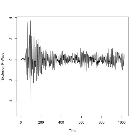
The eqexp object contains 17 columns corresponding to recording of 8 earthquake signals, 8 explosion signals and a final signal from "the Novaya Zemlya event of unknown origin". Each column consists of two signals: the P-wave which occupies the first 1024 entries, and the Q-wave which occupies the second 1024 entries. We will extract signal 14's P-wave (which corresponds to the explosion P-wave depicted in Nason (2013)) and then plot it.
exP <- eqexp[1:1024, 14]
ts.plot(exP)
This produces the plot above. The Priestley-Subba Rao (PSR) Test>
|