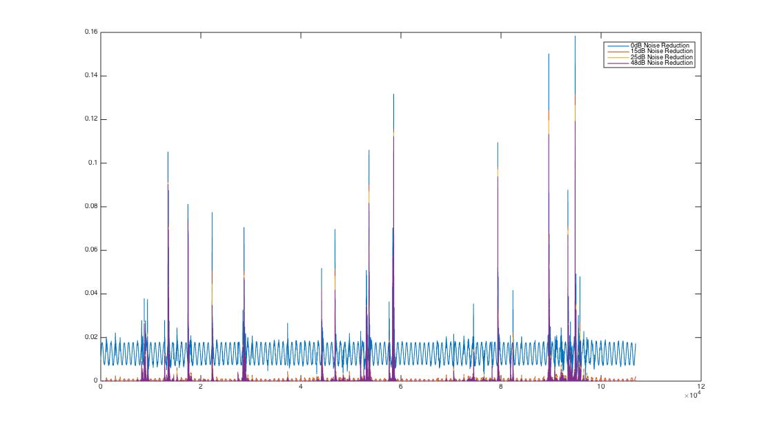
Acoustic data was acquired using the program Audacity at the standard sampling frequency 44100Hz, producing signals showing sound pressure level (SPL) over time. Background noise was removed by subtracting the noise profile from the signal. Different noise reduction levels were trialled on an example signal (see below) and a 48dB reduction proved most effective.
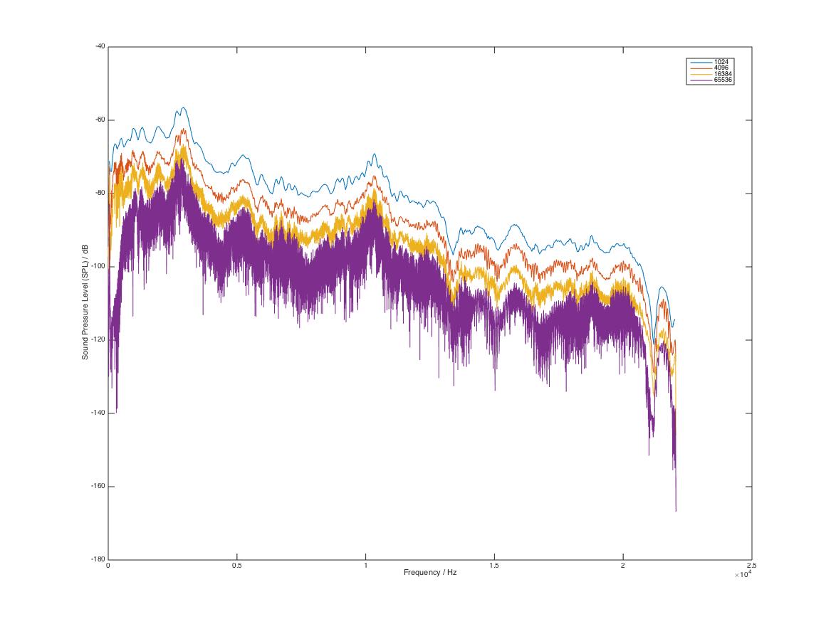
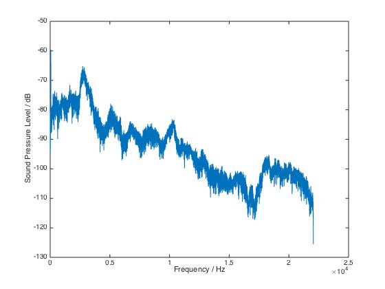
A Fast Fourier Transform (FFT) was computed on the signal to translate it to the frequency space. A Hanning window function was used for the spectrum and different sizes of FFT (number of frequency bins) were trialled to see which gave the most suitable frequency resolution (see first diagram below). A size of 16384 gave the best level of detail and was used for all FFTs (second diagram below gives a clear example).
The frequency spectrums were analysed in Matlab using a user-defined function that measures a number of acoustic parameters. The only input argument of this function is a threshold value that gives the minimum peak width for the ‘findpeak’ function contained within it. Indeed selecting an appropriate peak-finding metric was the biggest challenge here – many different ones were tested, but ‘minpeakwidth’ best identified significant peaks.
The following acoustic parameters were calculated from each spectrum:
- SPL of maximum frequency signal
- Maximum SPL
- Frequency of maximum SPL peak
- Ratio of SPL of maximum frequency peak and maximum SPL
- Total SPL
- Maximum frequency peak
- SPL of maximum frequency peak
- Width of maximum frequency peak
- Maximum peak width
- Frequency of maximum peak width
A one-way analysis of variance (1ANOVA) was performed (using the ‘anova1’ function in Matlab) for each of the above parameters. For those unfamiliar with 1ANOVA, it tests the null hypothesis that the mean of the three trials for each of the four days are equal to each other i.e. a certain acoustic parameter does not depend on the age of a Pringle. The result is a p-value, which if smaller than the significance level indicates that at least one of the three trial means is significantly different from the others. The most common significance levels are 0.05 or 0.01.
The resulting p-values for the acoustic parameters listed above ranged from 0.01-0.9, with only one parameter having a value below 0.05. This indicates the quality of the data is limited. One reason for this is likely due to the few number of trials (only three) carried out across the four days (sample sizes of around ten are common to most literature). However, the different p-values still give us a preliminary insight into perhaps the more significant acoustic parameters.
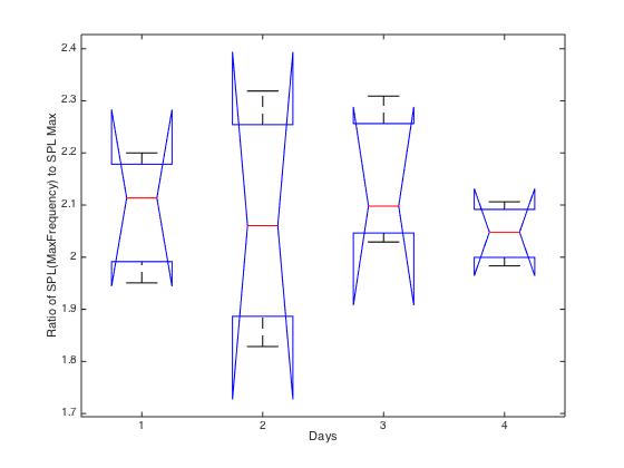
Acoustic parameters pertaining to the maximum frequency peak returned the smallest p-values. The SPL of the maximum frequency peak came out strongest with a p-value of 0.013 (see first box plot for this parameter below, compared with the second box plot which is for the ratio parameter – (4) in list above). The value for the maximum frequency peak and width of the maximum frequency peak were 0.022 and 0.354 respectively. Particular emphasis will be placed on these specific parameters in all further measurements.
 We would like to be able to measure the SPL and frequency distribution of sounds produced at force events to probe the correlation between the two (the main focus of much of the existing literature). We could also measure the fraction of mechanical energy released as sound during fracture events. An understanding of energy dissipation mechanisms and their variation across different materials is crucial to understanding how crispness emerges in different types of food. The main problem we face, however, is that the mechanical and acoustic data is currently acquired separately, meaning the two are not synced in time. This is the main focus for our development of the experimental method in preparation for the next set of measurements.
Our approach will then be to analyse a wide range of mechanical and acoustic parameters that are inter-related, such as the SPL at the first major fracture event, the number of sound peaks before and after the major fracture event etc. Then we will measure the correlation of each parameter with every other one to see which have the highest dependencies on one another.