In my last post I outlined our measuring equipment. We have since attached microphones to the equipment and have measured and recorded data for crisps. We started off looking at normal potato crisps, however, we soon realised that they were all different and it was impossible to get fair samples that only differed in age. We therefore, resorted to Pringles as they all have the same shape, texture and thickness.
We did measurements of singe Pringles to get a clear profile of the breaking but also did measurements with three Pringles stacked on top of each other to simulate a more realistic texture. We did three measurements for each configuration with fresh, one, two and three day old Pringles as well as Pringles which we steamed for a while to increase the moisture content.
The collection of data was faster than we had expected and we ended up with a lot of data which we had to analyse. To analyse it as efficiently as possible and to make sure our analysis techniques were consistent and fair we decided to write up several codes that would analyse the data. Sophia and I discussed what features we wanted to look at and wrote up code to do so. I concentrated mainly on the force and displacement features and Sophia analysed the sound data.
In the force channel we were mainly looking for small fractures as it has been asserted in existing papers that these might be what make up crispness. To find them I used a MATLAB script called peakfinder. I tuned it to be able to find even small peaks and put it in a code that used the peaks found by peakfinder to calculate the force drop of the peak and record it. The code would do this for all trials done on a specific data set (e.g. fresh single Pringles) and produce histograms by sorting the force drops into 20 equally spaced bins. The first figure shows an example of the graphs produced by this algorithm.
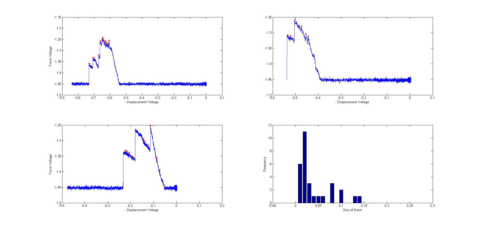
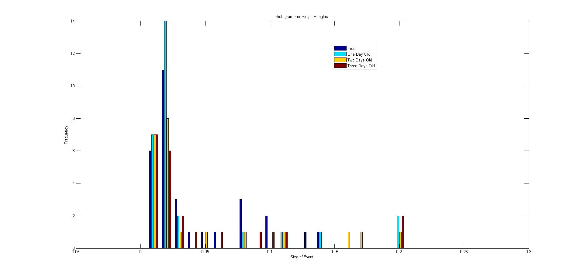
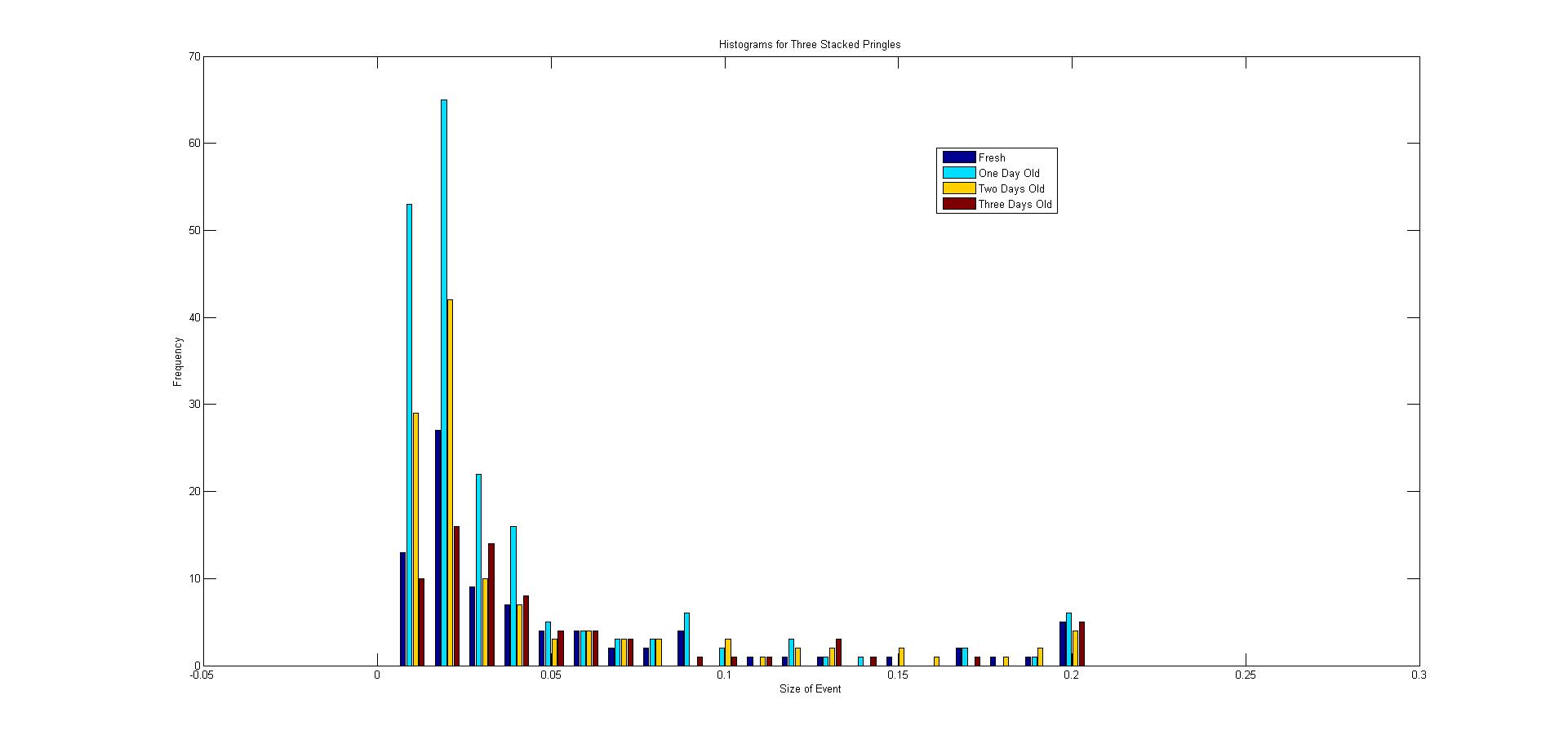
There seemed to be a qualitative trend of more medium sized peaks for fresher Pringles, however, it is hard to quantify this trend and to decide upon a weighing system based upon only four data sets. Once we move on to chips we can have many more data sets as there are more things we can vary and hence quantify and test trends more thoroughly. We will have the code to analyse this ready as soon as we do the measurements. The figures below show the histograms for all data sets for single Pringles as well as stacked Pringles
I also started to look at more features of the profile including the sum of the sizes of all force drops, the number of peaks before and after the maximum force drop, the maximum force recorded, the force at the peak at the maximum force drop and the size of the maximum drop. I searched this for all the measurements and then took an average for each data set. The feature that showed most dependence on age was the amount of force peaks after the major force drop. However, it is hard to tell if this is a trend or just happened by chance, based on such few measurements.
Sophia took Fast Fourier Transforms (FFTs) of the sound data and took automated readings of these. I cannot comment on the techniques used, but I can comment on the results found. The spectral feature that correlated most with the age of the Pringles was the nature of the peak with the highest frequency. With increasing age the centre, the amplitude and the width of this peak decreased in all four cases.
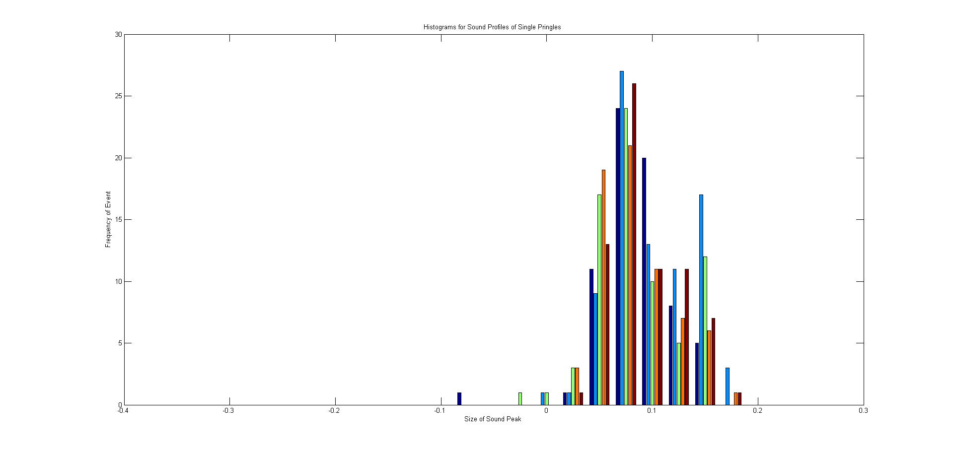
I also altered and applied my peak histogram code to the sound data in time space to try and see if there was a trend. The figure below shows the histograms for all the data. There seems to be not even a qualitative trend in the data but we haven’t correlated it with force and displacement yet and haven’t looked at other features in time space so not all information has been used yet. The diagram below shows the histograms for the sound profile of single Pringles.
One comment for “Update on our Progress – Automated Analysis Methods”